
The attention mechanism is the kingpin of the Transformer model. It drives the results, but runs the memory and time racket of \( O(L^2d) \), where \( L \) is input token count and \( d \) is the latent representation dimension.
The Reformer, Longformer and others attempted to topple it with \( O(L \log L ) \). Then there was this one model - Linformer they called him, and he had linear complexity. But he didn’t make it. Only recently published Performer done the job with \( O(L d^2 \log d ) \).

To prove that Performer is linear time with input token length increasing, forward and backward pass was measured.

How was that done? Read on, traveller! I will tell you a great story.
Not Paying for The Attention
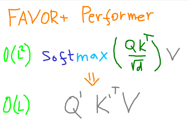
Original attention is a value vector weighted by softmax applied to dot product of key and query.
\( a_{\mathbf{orig}} = \mathbf{softmax}(\frac{QK^\intercal}{\sqrt{d}})V \)
The expensive the fact that I cannot decompose the softmax into a matrix multiplication to first multiply with the value matrix. Can we get a cheap estimate of that operation?
This Kernel Performs
I described a speed up using random features kernel approximation for word-movers distance in a previous post. In this case, the Performer approximates Transformer attention by kernelizing the softmax using positive orthogonal random features. Let’s define the kernel as a resulting elements of the softmax result also called attention matrix values as a function of corresponding query and key vectors - rows of query and key matricies.
\( k(Q_{i, \cdot }, K_{j, \cdot} ) = \) \( \mathbf{softmax}(\frac{Q K^\intercal}{\sqrt{d}})_{i, j} = \)
\( \mathbf{softmax}( \frac{ Q_{i, \cdot } K^{\intercal}_{j, \cdot} }{\sqrt{d}} ) \)
If we rescale the variables, we are looking to estimate exponential value of a dot product of two vectors.
\( \exp(x^\intercal y) = \) \( \exp(- \frac{\lVert x \rVert^2 + \lVert y \rVert^2}{2}) \exp(\frac{\lVert x+y \rVert^2}{2}) \)
The common way to estimate above function is using trigonometrical functions of random projection into vectors around zero. That runs into issues as the approximation has high variance around zero and can lead to negative values.
The authors of the paper instead propose alternative approximation using hyperbolical function, which are non-negative and don’t suffer from high variance. I give below a taste of derivation of the approximation.
How to draw random vectors in order to estimate the exponential of the dot product above?
\[ \exp(\frac{\lVert x+y \rVert^2}{2}) = \] \[ \exp(\frac{\lVert x+y \rVert^2}{2}) \int \exp(- \lVert \omega - (x+y) \rVert^2 / 2 ) \, \mathbf{d} \omega (2\pi)^{-d/2} = \] \[ \int \exp(\omega^\intercal (x + y)) \exp(- \lVert \omega \rVert^2 /2) \, \mathbf{d} \omega (2\pi)^{-d/2} = \] \[ \mathbb{E}_{\omega ~ N(0, 1)} \exp(\omega^\intercal (x+y)) \],
where \( \mathbb{E} \) is an expected over random vectors from a standard normal distribution. If we denote \( r \) as number of random vectors and expect the average to be close to an average, we intuit from below the softmax dot-product estimate.
\( k(x, y) \approx \) \( \sum_{i = 0}^r e^{\omega_i^\intercal x} e^{\omega_i^\intercal y} \)
In the full dimensionality, the dot-product would be replaced by matrix multiplication as teased in the intro.
Next, the proof uses isotropy of the standard normal distribution to invert sign of \( \omega \) on one half of the exponential, which results into hyperbolic cosine.
\( \mathbb{E} \exp(\omega^\intercal u) = \) \( \mathbb{E} \frac{ \exp(\omega^\intercal u) + \exp(- \omega^\intercal u)}{2} = \) \( \mathbb{E} \cosh (\omega^\intercal u) \ \)
How Many Random \( \omega \) to FAVOR+?
So do we just start sampling of the distro and hope for the best? No! If we make sure our random vectors (features) are orthogonal, while still being drawn from standard normal distribution, we can reduce how many we need them. The paper does this by drawing uniformly random orthogonal basis and then normalizing each row properly.
I am not clear however on the specifics here. But I think we first draw uniformly random vector components, removing the new vector projection to previously drawn vectors (Gramm-Schmidt orthogonalization method), and then normalize the vectors to make their squared norms match standard normal distribution vector norm (Maxwell-Boltzman distribution).
Doing this, the authors arrived at stronger guarantees of fast convergence and unbiasedness of the softmax estimate. The whole mechanism was then called FAVOR+.
Fast convergence implies that we need much less random features. In the Performer paper, they show very good performance on \( L = 4096, d = 16\) with feature count starting from 100. Their default setup was 256 features (Section A.3).
Out-performing
Perform over Linform
Linformer approximates attention with a low-rank matrix to achieve linear complexity \( O(L) \). Its strategy is to project key, value, and query matrices through into a low-dimensional space. It is unclear to me, in what way these projections are created. If randomly, then it is no surprise that Performer out-performs Linformer below.
Linformer approximates the matrix multiplications in contrast to Performer which approximates the Q and K multiplication and softmax at the same time. This difference gives Performer accuracy advantage over Linformer.
Both Linformer and Performer estimate attention using probabilistically drawn vectors (features). Apparently redrawing these helps training accuracy. I think this is a type of regularization method.

Perform over Reform
Reformer approximates attention with locality-sensitive hashing. It achieves complexity of \( O(L\log L) \). The hashing speeds up the calculation by only multiplying close angle keys and queries, which have high dot product.
Performer may have lower complexity, but does it is more powerful? The Perfomer’s authors provide comparison on image generation task, which requires a very large \( L \) in terms of bits-per-dimension (BPD ~ Log-likelihood).


